- The first assignment to x is a "useless" assignment, since the value computed for x is never used (and thus the first statement can be eliminated from the program).
- The expression 5 * 2 can be computed at compile time, simplifying the second assignment statement to x = 10;
- which variables are guaranteed to have constant values, and
- which variables will be used before being redefined.
- Forward problems (like constant propagation) where the information at a node n summarizes what can happen on paths from "enter" to n.
- Backward problems (like live-variable analysis), where the information at a node n summarizes what can happen on paths from n to "exit".
- What information holds at the start of the program.
- When a node n has more than one incoming edge in the CFG, how to combine the incoming information (i.e., given the information that holds after each predecessor of n, how to combine that information to determine what holds before n).
- How the execution of each node changes the information.
- a CFG,
- a domain D of "dataflow facts",
- a dataflow fact "init" (the information true at the start of the program for forward problems, or at the end of the program for backward problems),
- an operator ⌈⌉ (used to combine incoming information from multiple predecessors),
- for each CFG node n, a dataflow function fn : D → D (that defines the effect of executing n).
- The right-hand side has a variable that is not constant. In this case, the function result is the same as its input except that if variable x was constant the before n, it is not constant after n.
- All right-hand-side variables have constant values. In this case, the right-hand side of the assignment is evaluated producing consant-value c, and the dataflow-function result is the same as its input except that it includes the pair (x, c) for variable x (and excludes the pair for x, if any, that was in the input).
- the domain D of "dataflow facts",
- the operator ⌈⌉,
- the "init" dataflow fact,
- a dataflow function for each CFG node n.
Dataflow
Contents
Motivation for Dataflow Analysis
A compiler can perform some optimizations based only on local information. For example, consider the following code:
x = a + b;
x = 5 * 2;
It is easy for an optimizer to recognize that:
Some optimizations, however, require more "global" information. For example, consider the following code:
a = 1;
b = 2;
c = 3;
if (...) x = a + 5;
else x = b + 4;
c = x + 1;
In this example, the initial assignment to c (at line 3) is useless, and the expression x + 1 can be simplified to 7, but it is less obvious how a compiler can discover these facts since they cannot be discovered by looking only at one or two consecutive statements. A more global analysis is needed so that the compiler knows at each point in the program:
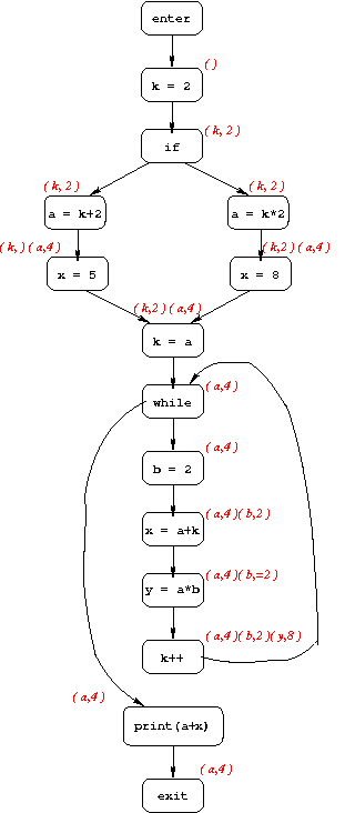
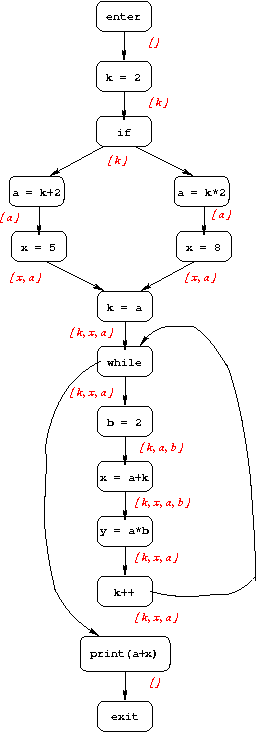
Examples of constant propagation and live-variable analysis
Below are examples illustrating two dataflow-analysis problems: constant propagation and live-variable analysis. Both examples use the following program:
1.   k = 2;
2.   if (...) {
3.     a = k + 2;
4.     x = 5;
5.   } else {
6.     a = k * 2;
7.     x = 8;
8.   }
9.   k = a;
10.  while (...) {
11.     b = 2;
12.     x = a + k;
13.     y = a * b;
14.     k++;
15.  }
16.  print(a+x);
Constant Propagation
The goal of constant propagation is to determine where in the program variables are guaranteed to have constant values. More specifically, the information computed for each CFG node n is a set of pairs, each of the form (variable, value). If we have the pair (x, v) at node n, that means that x is guaranteed to have value v whenever n is reached during program execution.
Below is the CFG for the example program, annotated with constant-propagation information.
Live-Variable Analysis
The goal of live-variable analysis is to determine which variables are "live" at each point in the program; a variable is live if its current value might be used before being overwritten. The information computed for each CFG node is the set of variables that are live immediately after that node. Below is the CFG for the example program, annotated with live variable information.
Draw the CFG for the following program, and annotate it with the constant-propagation and live-variable information that holds before each node.
N = 10;
k = 1;
prod = 1;
MAX = 9999;
while (k <= N) {
   read(num);
   if (MAX/num < prod) {
      print("cannot compute prod");
      break;
   }
   prod = prod * num;
   k++;
}
print(prod);
Defining a Dataflow Problem
Before thinking about how to define a dataflow problem, note that there are two kinds of problems:
Another way that many common dataflow problems can be categorized is as may problems or must problems. The solution to a "may" problem provides information about what may be true at each program point (e.g., for live-variables analysis, a variable is considered live after node n if its value may be used before being overwritten, while for constant propagation, the pair (x, v) holds before node n if x must have the value v at that point).
Now let's think about how to define a dataflow problem so that it's clear what the (best) solution should be. When we do dataflow analysis "by hand", we look at the CFG and think about:
This intuition leads to the following definition. An instance of a dataflow problem includes:
For constant propagation, an individual dataflow fact is a set of pairs of the form (var, val), so the domain of dataflow facts is the set of all such sets of pairs (the power set). For live-variable analysis, it is the power set of the set of variables in the program.
For both constant propagation and live-variable analysis, the "init" fact is the empty set (no variable starts with a constant value, and no variables are live at the end of the program).
For constant propagation, the combining operation ⌈⌉ is set intersection. This is because if a node n has two predecessors, p1 and p2, then variable x has value v before node n iff it has value v after both p1 and p2. For live-variable analysis, ⌈⌉ is set union: if a node n has two successors, s1 and s2, then the value of x after n may be used before being overwritten iff that holds either before s1 or before s2. In general, for "may" dataflow problems, ⌈⌉ will be some union-like operator, while it will be an intersection-like operator for "must" problems.
For constant propagation, the dataflow function associated with a CFG node that does not assign to any variable (e.g., a predicate) is the identity function. For a node n that assigns to a variable x, there are two possibilities:
For live-variable analysis, the dataflow function for each node n has the form: fn(S) = (S - KILLn) union GENn, where KILLn is the set of variables defined at node n, and GENn is the set of variables used at node n. In other words, for a node that does not assign to any variable, the variables that are live before n are those that are live after n plus those that are used at n; for a node that assigns to variable x, the variables that are live before n are those that are live after n except x, plus those that are used at n (including x if it is used at n as well as being defined there).
An equivalent way of formulating the dataflow functions for live-variable analysis is: fn(S) = (S intersect NOT-KILLn) union GENn, where NOT-KILLn is the set of variables not defined at node n. The advantage of this formulation is that it permits the dataflow facts to be represented using bit vectors, and the dataflow functions to be implemented using simple bit-vector operations (and or).
It turns out that a number of interesting dataflow problems have dataflow functions of this same form, where GENn and KILLn are sets whose definition depends only on n, and the combining operator ⌈⌉ is either union or intersection. These problems are called GEN/KILL problems, or bit-vector problems.
Consider using dataflow analysis to determine which variables might be used before being initialized; i.e., to determine, for each point in the program, for which variables there is a path to that point on which the variable was never defined. Define the "may-be-uninitialized" dataflow problem by specifying:
If you did not define the may-be-uninitialized problem as a GEN/KILL problem, go back and do that now (i.e., say what the GEN and KILL sets should be for each kind of CFG node, and whether ⌈⌉ should be union or intersection).