Table of Contents
- Overview
- Scanning
- Defining Syntax
- Syntax for Programming Languages
- Syntax-Directed Definition
- Abstract-Syntax Trees
- Parsing
- CYK Parsing
- LL(1) Parsing
- Shift/Reduce Parsing
- Syntax-Directed Translation (SDT)
- Symbol Tables
- Semantic Analysis
- Dataflow
- Dataflow Solving
- Types
- Runtime Environments
- Variable Access
- Parameter Passing
- Code Generation
- Welcome
- Introduction
- The Scanner
- The Parser
- The Semantic Analyzer
- The Intermediate Code Generator
- The Optimizer
- The Code Generator
- A recognizer of some source language S.
- A translator (of programs written in S into programs written in some object or target language T).
- A program written in some host language H
- The scanner groups the characters into lexemes (sequences of characters that "go together").
- Each lexeme corresponds to a token; the scanner forwards each token (plus maybe some additional information, such as a position within at which the token was found in the input file) to the parser.
- Groups tokens into "grammatical phrases", discovering the underlying structure of the source program.
- Finds syntax errors. For example, the source code
could correspond to the sequence of tokens:
5 position = ;intlit id assign semicolonAll are legal tokens, but that sequence of tokens is erroneous. - Might find some "static semantic" errors, e.g., a use of an undeclared variable, or variables that are multiply declared.
- Might generate code, or build some intermediate representation of the program such as an abstract-syntax tree.
- The interior nodes of the tree are operators.
- A node's children are its operands.
- Each subtree forms a "logical unit", e.g., the subtree with * at its root shows that because multiplication has higher precedence than addition, this operation must be performed as a unit (not initial+rate).
- The assembler transforms an assembly code file (such as one produced by the compiler) into a relocatable, which is either an object file (typically given the .o extension) or a library (typically given the .so or .a extension, for a dynamically-linked or statically-linked library, respectively).
- The linker merges the various object files and static libraries output by the assembler into a single executable.
- Overview
- Finite-State Machines
- Regular Expressions
- Using Regular Expressions and Finite-State Machines to Define a Scanner
- A compiler recognizes legal programs in some (source) language.
- A finite-state machine recognizes legal strings in some language.
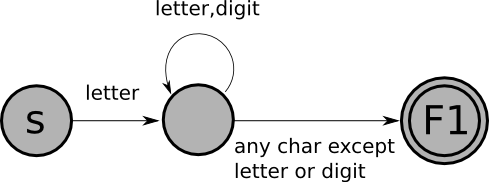
- Nodes are states.
- Edges (arrows) are transitions. Each edge should be labeled with a single character. In this example, we've used a single edge labeled "letter" to stand for 52 edges labeled 'a', 'b', $\ldots$, 'z', 'A', $\ldots$, 'Z'. (Similarly, the label "letter,digit" stands for 62 edges labeled 'a',...'Z','0',...'9'.)
- S is the start state; every FSM has exactly one (a standard convention is to label the start state "S").
- A is a final state. By convention, final states are drawn using a double circle, and non-final states are drawn using single circles. A FSM may have more than one final state.
- The FSM starts in its start state.
- If there is a edge out of the current state whose label matches the current input character, then the FSM moves to the state pointed to by that edge, and "consumes" that character; otherwise, it gets stuck.
- The finite-state machine stops when it gets stuck or when it has consumed all of the input characters.
- The entire string is consumed (the machine did not get stuck), and
- the machine ends in a final state.
xtmp2XyZzyposition27123a?13apples- a sequence of one or more letters and/or digits,
- followed by an at-sign,
- followed by one or more letters,
- followed by zero or more extensions.
- An extension is a dot followed by one or more letters.
- $Q$ is a finite set of states ($\{\mathrm{S,A,B}\}$ in the above example).
- $\Sigma$ (an uppercase sigma) is the alphabet of the machine, a finite set of characters that label the edges ($\{+,-,0,1,...,9\}$ in the above example).
- $q$ is the start state, an element of $Q$ ($\mathrm{S}$ in the above example).
- $F$ is the set of final states, a subset of $Q$ ({B} in the above example).
- $\delta$ is the state transition relation: $Q \times \Sigma \rightarrow Q$ (i.e., it is a function that takes two arguments -- a state in $Q$ and a character in $\Sigma$ -- and returns a state in $Q$).
- Deterministic:
- No state has more than one outgoing edge with the same label.
- Non-Deterministic:
- States may have more than one outgoing edge with same label.
- Edges may be labeled with $\varepsilon$ (epsilon), the empty string. The FSM can take an $\varepsilon$-transition without looking at the current input character.
- Have a variable named state, initialized to S (the start state).
- Repeat:
- read the next character from the input
- use the table to assign a new value to the state variable
- $\mathrm{digit} \; | \; \mathrm{letter} \; \mathrm{letter}$
- $\mathrm{digit} \; | \; \mathrm{letter} \; \mathrm{letter}$*
- $\mathrm{digit} \; | \; \mathrm{letter}$*
- ID + ID
- ID * ID
- ID == ID
- The scanner sometimes needs to look one or more characters
beyond
the last character of the current token, and then needs to "put
back" those characters so that the next time the scanner is called
it will have the correct current character.
For example, when scanning a program written in the simple
assignment-statement language defined above, if the input is
"==", the scanner should return the EQUALS token, not two ASSIGN
tokens. So if the current character is "=", the scanner must
look at the next character to see whether it is another "="
(in which case it will return EQUALS), or is some other character
(in which case it will put that character back and return ASSIGN).
- It is no longer correct to run the FSM program until the machine gets stuck or end-of-input is reached, since in general the input will correspond to many tokens, not just a single token.
- modify the machines so that a state can have an associated action to "put back N characters" and/or to "return token XXX",
- we must combine the finite-state machines for all of the tokens in to a single machine, and
- we must write a program for the "combined" machine.
- The table will include a column for end-of-file as well as for all possible characters (the end-of-file column is needed, for example, so that the scanner works correctly when an identifier is the last token in the input).
- Each table entry may include an action as well as or instead of a new state.
- Instead of repeating "read a character; update the state variable" until the machine gets stuck or the entire input is read, the code will repeat: "read a character; perform the action and/or update the state variable" (eventually, the action will be to return a value, so the scanner code will stop, and will start again in the start state next time it is called).
- Overview
- Example: Simple Arithmetic Expressions
- Formal Definition
- Example: Boolean Expressions, Assignment Statements, and If Statements
- Self-Study #1
- The Language Defined by a CFG
- Groups the tokens into "grammatical phrases".
- Discovers the underlying structure of the program.
- Finds syntax errors.
- Perhaps also performs some actions to find other kinds of errors.
- an abstract-syntax tree (maybe + a symbol table),
- or intermediate code,
- or object code.
- An integer is an arithmetic expression.
- If exp1 and exp2 are arithmetic expressions,
then so are the following:
- exp1 - exp2
- exp1 / exp2
- ( exp1 )
- The grammar has five terminal symbols: intliteral minus divide lparen rparen. The terminals of a grammar used to define a programming language are the tokens returned by the scanner.
- The grammar has one nonterminal: Exp (note that a single name, Exp, is used instead of Exp1 and Exp2 as in the English definition above).
- The grammar has four productions or rules,
each of the form:
Exp $\longrightarrow$ ...A production left-hand side is a single nonterminal. A production right-hand side is either the special symbol $\varepsilon$ (the same $\varepsilon$ that can be used in a regular expression) or a sequence of one or more terminals and/or nonterminals (there is no rule with $\varepsilon$ on the right-hand side in the example given above).
- $N$ is a set of nonterminals.
- $\Sigma$ is a set of terminals.
- $P$ is a set of productions (or rules).
- $S$ is the start nonterminal (sometimes called the goal nonterminal) in $N$. If not specified, then it is the nonterminal that appears on the left-hand side of the first production.
- "true" is a boolean expression, recognized by the token true.
- "false" is a boolean expression, recognized by the token false.
- If exp1 and exp2 are boolean expressions, then so are the following:
- exp1 || exp2
- exp1 && exp2
- ! exp1
- ( exp1 )
- The word "if", followed by a boolean expression in parentheses, followed by a statement, or
- The word "if", followed by a boolean expression in parentheses, followed by a statement, followed by the word "else", followed by a statement.
- Start by setting the "current sequence" to be the start nonterminal.
- Repeat:
- find a nonterminal $X$ in the current sequence;
- find a production in the grammar with $X$ on the left (i.e., of the form $X$ → $\alpha$, where $\alpha$ is either $\varepsilon$ (the empty string) or a sequence of terminals and/or nonterminals);
- Create a new "current sequence" in which $\alpha$ replaces the $X$ found above;
- $\Longrightarrow$ means derives in one step
- $\stackrel{+}\Longrightarrow$ means derives in one or more steps
- $\stackrel{*}\Longrightarrow$ means derives in zero or more steps
- $S$ is the start nonterminal of $G$
- $w$ is a sequence of terminals or $\varepsilon$
- Start with the start nonterminal.
- Repeat:
- choose a leaf nonterminal $X$
- choose a production $X \longrightarrow \alpha$
- the symbols in $\alpha$ become the children of $X$ in the tree
- Overview
- Ambiguous Grammars
- Disambiguating Grammars
- List Grammars
- A Grammar for a Programming Language
- Summary
- more than one leftmost derivation of $w$ or,
- more than one rightmost derivation of $w$, or
- more than one parse tree for $w$
- A grammar is recursive in nonterminal $X$ if: $$X \stackrel{+}\longrightarrow{\Tiny\dots\,}X{\Tiny\,\dots}$$ (in one or more steps, $X$ derives a sequence of symbols that includes an $X$).
- A grammar is left recursive in $X$ if: $$X \stackrel{+}\longrightarrow X{\Tiny\,\dots}$$ (in one or more steps, $X$ derives a sequence of symbols that starts with an $X$).
- A grammar is right recursive in $X$ if: $$X \stackrel{+}\longrightarrow {\Tiny\dots\,}X$$ (in one or more steps, $X$ derives a sequence of symbols that ends with an $X$).
- For left associativity, use left recursion.
- For right associativity, use right recursion.
- One or more PLUSes (without any separator or terminator).
(Remember, any of the following three grammars defines
this language; you don't need all three lines).
- xList $\longrightarrow$ PLUS | xList xList
- xList $\longrightarrow$ PLUS | xList PLUS
- xList $\longrightarrow$ PLUS | PLUS xList
- One or more runs of one or more PLUSes, each run separated by commas:
- xList $\longrightarrow$ PLUS | xList COMMA xList
- xList $\longrightarrow$ PLUS | xList COMMA PLUS
- xList $\longrightarrow$ PLUS | PLUS COMMA xList
- One or more PLUSes, each PLUS terminated by a semi-colon:
- xList $\longrightarrow$ PLUS SEMICOLON | xList xList
- xList $\longrightarrow$ PLUS SEMICOLON | xList PLUS SEMICOLON
- xList $\longrightarrow$ PLUS SEMICOLON | PLUS SEMICOLON xList
- Zero or more PLUSes (without any separator or terminator):
- xList $\longrightarrow$ $\varepsilon$ | PLUS | xList xList
- xList $\longrightarrow$ $\varepsilon$ | PLUS | xList PLUS
- xList $\longrightarrow$ $\varepsilon$ | PLUS | PLUS xList
- Zero or more PLUSes, each PLUS terminated by a semi-colon:
- xList $\longrightarrow$ $\varepsilon$ | PLUS SEMICOLON | xList xList
- xList $\longrightarrow$ $\varepsilon$ | PLUS SEMICOLON | xList PLUS SEMICOLON
- xList $\longrightarrow$ $\varepsilon$ | PLUS SEMICOLON | PLUS SEMICOLON xList
-
The trickiest kind of list is a list of
zero or more x's, separated by commas.
To get it right, think of the definition as follows:
-
Either an empty list, or a non-empty list of x's separated
by commas.
xList $\longrightarrow$ $\varepsilon$ | nonemptyList nonemptyList $\longrightarrow$ PLUS | PLUS COMMA nonemptyList
Overview
Hello, and welcome to the course readings for Drew Davidson's EECS 665, "Compiler Construction". This set of course notes has been shaped by me (Drew) in order to serve as a written companion to the course lectures and discussions offered as part of EECS665. As such, it's written pretty informally, and will often draw on my personal observations and experience. These readings are not intended to serve as a standalone reference for compiler topics or as a guide for building a compiler. Thus, I'll start these readings with a disclaimer exactly opposite of most textbooks: it is not for a general audience, and it is intended to be read straight through from start to back.
Some additional disclaimers: In the interest of brevity, these readings will occasionally adopt a definition and stick to it without fully exploring alternative definitions, or considering all implications of the definition. If you feel that a superior definition exists, please do let me know. Furthermore, the readings constitute a living document, updated and refined when possible. If you see a typo, mistake, or even just something where you'd like some more writing, please do let me know.
While much of the material in the course readings has been updated, modified, or written by me, it is based originally on a set of readings created by Susan Horwitz at the University of Wisconsin-Madison. In the interest of providing the best possible guide to the subject, I will frequently read or re-read classic textbooks on compilers, and whatever course materials from other classes might be floating around on the internet. It is my intention to synthesize this information and provide wholly original material herein. That being said, if you see an example or text in the readings that you feel has not been appropriately credited to an external source, please contact me at your earliest convenience so that we can arrange for the material to be taken down, cited, or come to another arrangement.
IntroductionWhat is a compiler? A common answer amongst my students is something like "A program that turn code into a program", which is honestly not bad (if a bit imprecise). Without dwelling overly much on the messy details, let's refine this definition and run with it. For this class, we'll say that a compiler is:
Here's a simple pictorial view:
A compiler operates in phases; each phase translates the source program from one representation to another. Different compilers may include different phases, and/or may order them somewhat differently. A typical organization is shown below.
Below, we look at each phase of the compiler, giving a high-level overview of how
the code snippet position = initial + rate + 60 is represented
throughout the above workflow.
The Scanner
The scanner performs lexical analysis, which means to group the input characters into the fundamental units of the source language. If some character(s) of input fails to correspond to a valid group, the scanner may also report lexical errors.
Some terminology for lexical analysis:
The definitions of what is a lexeme, token, or bad character all depend on the source language.
Example 1
Here are some C-like lexemes and the corresponding tokens:
lexeme:                   ;           =        index      tmp      37       102

corresponding token:  semicolon     assign       id        id       intlit     intlit
Note that multiple lexemes can correspond to the same token (e.g., the index and tmp
lexemes both correspond to id tokens.
Example 2 (the running example)
Given the source code:
position = initial + rate * 60 ;
a C-like scanner would return the following sequence of tokens:
id assign id plus id times intlit semicolon
The errors that a scanner might report are usually due to characters that cannot be a valid part of any token.
Erroneous characters for Java source include hash (#) and control-a.
Erroneous characters for C source include the carat (^).
The Parser
The parser performs syntactic analysis, which means to group the tokens of the language into constructs of the programming language (such as loops, expressions, functions, etc). A good analogy is to think of the scanner as building the "words" of the programming language, and the parser as building the "sentences" or "grammatical phrases" of the source program.
Example
source code: position = initial + rate * 60 ;
Abstract syntax tree:
Key features of the Abstract-Syntax Tree (AST):
While the above presentation has implied that syntactic analysis comes strictly after lexical analysis has been completed, the two phases can often be interleaved, with the parser serving as the "driver" module: the parser sends requests to the lexical analysis to produce one token at a time, which is then added to the AST or rejected if syntactically invalid. Thus, the AST is built incrementally. One reason for this behavior is that if problems are detected early in the parse, the compiler can emit an error quickly. This "fail-fast" behavior is a major design goal in compiler construction, as it can save users time and compute cycles.
The semantic analyzer checks for (more) "static semantic" errors, e.g., type errors. It may also annotate and/or change the abstract syntax tree (e.g., it might annotate each node that represents an expression with its type).
Example:
Abstract syntax tree before semantic analysis:

Abstract syntax tree after semantic analysis:
The Intermediate Code Generator
The intermediate code generator translates from abstract-syntax tree
to intermediate code.
One possibility is 3-address code (code in which each instruction
involves at most 3 operands).
Below is an example of 3-address code for the abstract-syntax tree
shown above.
Note that in this example, the second and third instructions each have
exactly three operands (the location where the result of the
operation is stored, and two operators);
the first and fourth instructions have just two operands ("temp1" and "60"
for instruction 1, and "position" and "temp3" for instruction 4).
The Optimizer
The optimizer tries to improve code generated by the intermediate code
generator.
The goal is usually to make code run faster, but the optimizer may also
try to make the code smaller.
In the example above, an optimizer might first discover that the
conversion of the integer 60 to a floating-point number can be done
at compile time instead of at run time.
Then it might discover that there is no need for "temp1" or "temp3".
Here's the optimized code:
The Code Generator
The code generator generates assembly code from (optimized)
intermediate code. For example, the following x64 code might
be generated for our running example:
It's worth noting that the above representation of the running
example is still a text file, though one that the compiler
proper considers to be the final output. There is still work
left to be done before we have an executable program. Usually,
a collection of programs, collectively referred
to as a compiler toolchain, work in sequence to build the
executable:
When it comes time for the program to
actually be run, the loader maps the executable
file into memory (alongside whatever dynamic libraries
may be required) as a process, and then hands control
to the operating system to actually begin execution
of the program. In modern workstation computing, the loader
is integrated into the Operating System, but in some
legacy, specialized, and embedded systems the loader is still
a distinct program.
Students who use compilers like gcc or llvm are often
surprised at the existence of distinct "post-compilation"
steps to produce an executable. Indeed the term "compiler"
is often used to refer to the full "compiler toolchain".
Nevertheless, the workflow from compilation, to assembly, to
linkage, is represented as a series of distinct
modules within many popular compilers, and each of the tools
can be invoked separately. For example, running the
toolchain for C gcc can be accomplished using cc (the c
compiler proper), as (the gnu assembler), and
ld (the gnu linker).
		temp1 = inttofloat(60)
		temp2 = rate * temp1
		temp3 = initial + temp2
		position = temp3
		temp2 = rate * 60.0
		position = initial + temp2
        movl    rate(%rip), %eax
        imull   $60, %eax, %edx
        movl    initial(%rip), %eax
        addl    %edx, %eax
        movl    %eax, position(%rip)
Scanning
OverviewL
Recall that the job of the scanner is to translate the sequence of characters that is the input to the compiler to a corresponding sequence of tokens. In particular, each time the scanner is called it should find the longest sequence of characters in the input, starting with the current character, that corresponds to a token, and should return that token.
It is possible to write a scanner from scratch, but it is often much easier and less error-prone approach is to use a scanner generator like lex or flex (which produce C or C++ code), or jlex (which produces java code). The input to a scanner generator includes one regular expression for each token (and for each construct that must be recognized and ignored, such as whitespace and comments). Therefore, to use a scanner generator you need to understand regular expressions. To understand how the scanner generator produces code that correctly recognizes the strings defined by the regular expressions, you need to understand finite-state machines (FSMs).
Finite State MachinesLA finite-state machine is similar to a compiler in that:
In both cases, the input (the program or the string) is a sequence of characters.
Here's an example of a finite-state-machine that recognizes Pascal identifiers (sequences of one or more letters or digits, starting with a letter):
In this picture:
A FSM is applied to an input (a sequence of characters). It either accepts or rejects that input. Here's how the FSM works:
An input string is accepted by a FSM if:
The language defined by a FSM is the set of strings accepted by the FSM.
The following strings are in the language of the FSM shown above:
The following strings are not in the language of the FSM shown above:
Write a finite-state machine that accepts e-mail addresses, defined as follows:
Let us consider another example of an FSM:
Example: Integer LiteralsLThe following is a finite-state machine that accepts integer literals with an optional + or - sign:
Formal Definition
An FSM is a 5-tuple: $(Q,\Sigma,\delta,q,F)$
Here's a definition of $\delta$ for the above example, using a state transition table:
| + | - | $\mathrm{digit}$ | |
| $S$ | $A$ | $A$ | $B$ |
| $A$ | $B$ | ||
| $B$ | $B$ |
Deterministic and Non-Deterministic FSMsL
There are two kinds of FSM:
Example
Here is a non-deterministic finite-state machine that recognizes the same language as the second example deterministic FSM above (the language of integer literals with an optional sign):
Sometimes, non-deterministic machines are simpler than deterministic ones, though not in this example.
A string is accepted by a non-deterministic finite-state machine if there exists a sequence of moves starting in the start state, ending in a final state, that consumes the entire string. For example, here's what happens when the above machine is run on the input "+75":
| After scanning | Can be in these states | ||
| (nothing) | $S$ | $A$ | |
| $+$ | $A$ | (stuck) | |
| $+7$ | $B$ | (stuck) | |
| $+75$ | $B$ | (stuck) | |
It is worth noting that there is a theorem that says:
-
For every non-deterministic finite-state machine $M$,
there exists a deterministic machine $M'$ such that $M$ and
$M'$ accept the same language.
How to Implement a FSM
The most straightforward way to program a (deterministic) finite-state machine is to use a table-driven approach. This approach uses a table with one row for each state in the machine, and one column for each possible character. Table[j][k] tells which state to go to from state j on character k. (An empty entry corresponds to the machine getting stuck, which means that the input should be rejected.)
Recall the table for the (deterministic) "integer literal" FSM given above:
| + | - | $\mathrm{digit}$ | |
| $S$ | $A$ | $A$ | $B$ |
| $A$ | $B$ | ||
| $B$ | $B$ |
The table-driven program for a FSM works as follows:
Regular Expressions
Regular expressions provide a compact way to define a language that can be accepted by a finite-state machine. Regular expressions are used in the input to a scanner generator to define each token, and to define things like whitespace and comments that do not correspond to tokens, but must be recognized and ignored.
As an example, recall that a Pascal identifier consists of a letter, followed by zero or more letters or digits. The regular expression for the language of Pascal identifiers is:
-
letter . (letter | digit)*
| | | means "or" |
| . | means "followed by" |
| * | means zero or more instances of |
| ( ) | are used for grouping |
Often, the "followed by" dot is omitted, and just writing two things next to each other means that one follows the other. For example:
-
letter (letter | digit)*
In fact, the operands of a regular expression should be single characters or the special character epsilon, meaning the empty string (just as the labels on the edges of a FSM should be single characters or epsilon). In the above example, "letter" is used as a shorthand for:
-
a | b | c | ... | z | A | ... | Z
To understand a regular expression, it is necessary to know the precedences of the three operators. They can be understood by analogy with the arithmetic operators for addition, multiplication, and exponentiation:
| Regular Expression Operator |
Analogous Arithmetic Operator |
Precedence |
| | | plus | lowest precedence |
| . | times | middle |
| * | exponentiation | highest precedence |
So, for example, the regular expression:
-
$\mathrm{letter}.\mathrm{letter} | \mathrm{digit}\mathrm{^*}$
-
$(\mathrm{letter}.\mathrm{letter}) | (\mathrm{digit}\mathrm{^*})$
Describe (in English) the language defined by each of the following regular expressions:
Example: Integer LiteralsL
Let's re-examine the example of integer literals for regular-expressions:
An integer literal with an optional sign can be defined in English as:
The corresponding regular expression is:
Note that the regular expression for "one or more digits" is:
i.e., "one digit followed by zero or more digits". Since "one or more" is a common pattern, another operator, +, has been defined to mean "one or more". For example, $\mathrm{digit}$+ means "one or more digits", so another way to define integer literals with optional sign is:
The Language Defined by a Regular ExpressionL
Every regular expression defines a language: the set of strings that match the expression. We will not give a formal definition here, instead, we'll give some examples:
| Regular Expression | Corresponding Set of Strings | |
| $\varepsilon$ | $\{$""$\}$ | |
| a | $\{$"a"$\}$ | |
| a.b.c | $\{$"abc"$\}$ | |
| a | b | c | $\{$"a", "b", "c"$\}$ | |
| (a | b | c)* | $\{$"", "a", "b", "c", "aa", "ab", $\ldots$, "bccabb", $\ldots$ $\}$ |
Using Regular Expressions and FSMs to Define a ScannerL
There is a theorem that says that for every regular expression, there is a finite-state machine that defines the same language, and vice versa. This is relevant to scanning because it is usually easy to define the tokens of a language using regular expressions, and then those regular expression can be converted to finite-state machines (which can actually be programmed).
For example, let's consider a very simple language: the language of assignment statements in which the left-hand side is a Pascal identifier (a letter followed by one or more letters or digits), and the right-hand side is one of the following:
| Token | Regular Expression |
| assign | "=" |
| id | letter (letter | digit)* |
| plus | "$+$" |
| times | "$*$" |
| equals | "="."=" |
These regular expressions can be converted into the following finite-state machines:
| assign: | |
| id: | |
| plus: | |
| times: | |
| equals: |
Given a FSM for each token, how do we write a scanner? Recall that the goal of a scanner is to find the longest prefix of the current input that corresponds to a token. This has two consequences:
Furthermore, remember that regular expressions are used both to define tokens and to define things that must be recognized and skipped (like whitespace and comments). In the first case a value (the current token) must be returned when the regular expression is matched, but in the second case the scanner should simply start up again trying to match another regular expression.
With all this in mind, to create a scanner from a set of FSMs, we must:
For example, the FSM that recognizes Pascal identifiers must be
modified as follows:
with the following table of actions:
F1: put back 1 char, return ID
And here is the combined FSM for the five tokens (with the actions noted below):
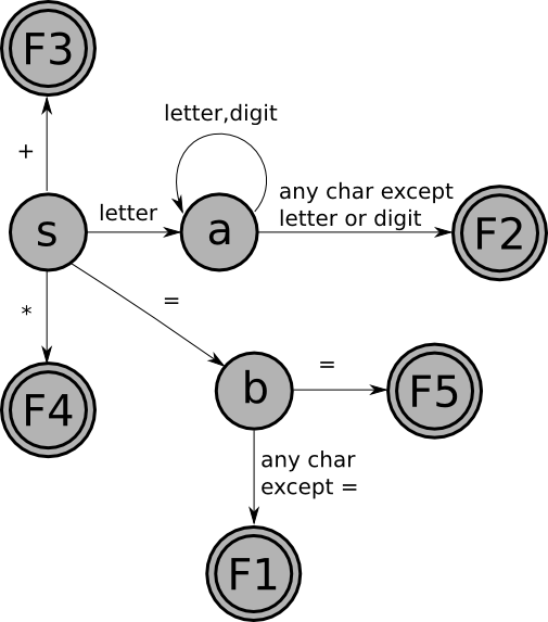
with the following table of actions:
F1: put back 1 char; return assign
F2: put back 1 char; return id
F3: return plus
F4: return times
F5: return equals
We can convert this FSM to code using the table-driven technique described above, with a few small modifications:
| + | * | = | $\mathrm{letter}$ | $\mathrm{digit}$ | EOF | |
| $S$ | return plus | return times | $B$ | $A$ | ||
| $A$ | put back 1 char; return id |
put back 1 char; return id |
put back 1 char; return id |
$A$ | $A$ | return id |
| $B$ |
put back 1 char; return assign |
put back 1 char; return assign |
return equals |
put back 1 char; return assign |
put back 1 char; return assign |
return assign |
Suppose we want to extend the very simple language of assignment statements defined above to allow both integer and double literals to occur on the right-hand sides of the assignments. For example:
would be a legal assignment.
What new tokens would have to be defined? What are the regular expressions, the finite-state machines, and the modified finite-state machines that define them? How would the the "combined" finite-state machine given above have to be augmented?
Defining Syntax
Contents
Recall that the input to the parser is a sequence of tokens (received interactively, via calls to the scanner). The parser:
The output depends on whether the input is a syntactically legal program; if so, then the output is some representation of the program:
We know that we can use regular expressions to define languages (for example, the languages of the tokens to be recognized by the scanner). Can we use them to define the language to be recognized by the parser? Unfortunately, the answer is no. Regular expressions are not powerful enough to define many aspects of a programming language's syntax. For example, a regular expression cannot be used to specify that the parentheses in an expression must be balanced, or that every ``else'' statement has a corresponding ``if''. Furthermore, a regular expression doesn't say anything about underlying structure. For example, the following regular expression defines integer arithmetic involving addition, subtraction, multiplication, and division:
digit+ (("+" | "-" | "*" | "/") digit+)*
Example: Simple Arithmetic ExpressionsL
We can write a context-free grammar (CFG) for the language of (very simple) arithmetic expressions involving only subtraction and division. In English:
Exp$\;\longrightarrow\;$ Exp minus Exp
Exp$\;\longrightarrow\;$ Exp divide Exp
Exp$\;\longrightarrow\;$ lparen Exp rparen
And here is how to understand the grammar:
A more compact way to write this grammar is:
Intuitively, the vertical bar means "or", but do not be fooled into thinking that the right-hand sides of grammar rules can contain regular expression operators! This use of the vertical bar is just shorthand for writing multiple rules with the same left-hand-side nonterminal.
Formal DefinitionLA CFG is a 4-tuple $\left( N, \Sigma, P, S \right)$ where:
Example: Boolean Expressions, Assignment Statements, and If StatementsL
The language of boolean expressions can be defined in English as follows:
BExp$\;\longrightarrow\;$false
BExp $\;\longrightarrow\;$ BExp or BExp
BExp $\;\longrightarrow\;$ BExp and BExp
BExp $\;\longrightarrow\;$ not BExp
BExp $\;\longrightarrow\;$ lparen BExp rparen
Here is a CFG for a language of very simple assignment statements (only statements that assign a boolean value to an identifier):
-
Stmt $\;\longrightarrow\;$
id
assign
BExp
semicolon
We can "combine" the two grammars given above, and add two more rules to get a grammar that defines a language of (very simple) if-statements. In words, an if-statement is:
Here is the combined context-free grammar:
Stmt $\;\longrightarrow\;$ if lparen BExp rparen Stmt else Stmt
Stmt $\;\longrightarrow\;$ id assign BExp semicolon
BExp $\;\longrightarrow\;$ true
BExp $\;\longrightarrow\;$ false
BExp $\;\longrightarrow\;$ BExp or BExp
BExp $\;\longrightarrow\;$ BExp and BExp
BExp $\;\longrightarrow\;$ not BExp
BExp $\;\longrightarrow\;$ lparen BExp rparen
Write a context-free grammar for the language of very simple while loops (in which the loop body only contains one statement) by adding a new production with nonterminal stmt on the left-hand side.
The language defined by a context-free grammar is the set of strings (sequences of terminals) that can be derived from the start nonterminal. What does it mean to derive something?
Thus, we arrive either at $\varepsilon$ or at a string of terminals. That is how we derive a string in the language defined by a CFG.
Below is an example derivation, using the 4 productions for the grammar of arithmetic expressions given above. In this derivation, we use the actual lexemes instead of the token names (e.g., we use the symbol "-" instead of minus).
-
Exp
$\Longrightarrow$ Exp - Exp$\Longrightarrow$ 1 - Exp$\Longrightarrow$ 1 - Exp / Exp$\Longrightarrow$ 1 - Exp / 2
$\Longrightarrow$ 1 - 4 / 2
And here is some useful notation:
So, given the above example, we could write: Exp $\stackrel{+}\Longrightarrow$ 1 - Exp / Exp.
A more formal definition of what it means for a CFG $G$ to define a language may be stated as follows:
where
There are several kinds of derivations that are important. A derivation is a leftmost derivation if it is always the leftmost nonterminal that is chosen to be replaced. It is a rightmost derivation if it is always the rightmost one.
Parse TreesLAnother way to derive things using a context-free grammar is to construct a parse tree (also called a derivation tree) as follows:
Here is the example expression grammar given above:
and, using that grammar, here's a parse tree for the string 1 - 4 / 2:
Stmt $\;\longrightarrow\;$ if lparen BExp rparen Stmt else Stmt
Stmt $\;\longrightarrow\;$ id assign BExp semicolon
BExp $\;\longrightarrow\;$ true
BExp $\;\longrightarrow\;$ false
BExp $\;\longrightarrow\;$ BExp or BExp
BExp $\;\longrightarrow\;$ BExp and BExp
BExp $\;\longrightarrow\;$ not BExp
BExp $\;\longrightarrow\;$ lparen BExp rparen
Question 2: Give a parse tree for the same string.
Syntax for Programming Languages
Contents
While our primary focus in this course is compiler development, we will necessarily touch on some of the aspects of programming language development in the process. A programming language needs to define what constitutes valid syntax for the language (i.e. language definition). The compiler needs to determine whether a given stream of tokens belongs[1] During parsing, we're only interested in capturing the syntax (as opposed to the semantics) of the programming language. The syntax of a programming language is intuitively understood to be the structure of the code, whereas sematics is the meaning of the code. to that language (i.e. language recognition). Conveniently, a sufficiently rigorous definition of the language can be used as the basis of a recognizer: if there is some way to produce a given string according to the definition of the language, then it is necessarily part of the language.
Context-free Grammars (CFGs) provide a promising basis for defining the syntax of a programming language: For one, the class of languages that CFGs recognize (the context-free languages) are expressive enough to capture popular syntactic constructs. At the same time, CFGs are (relatively) uniform and compact. As such, programmers are expected to be able to read a CFG-like definition of a language and recognize whether or not a given string of input tokens belongs that language.
For a compiler, however, performing language recognition (making a yes/no determination of whether a string belongs to a language) is not enough to complete syntactic analysis. In order for a context-free grammar to serve as a suitable definition for a programming language, there are a number of refinements that need to be considered. In this section, we will discuss some of these considerations.
We'll caveat the claim that "CFGs are a good way to define programming-language syntax" at the end of this reading, but it's worth noting that there are some compelling arguments to the contrary for practical purposes.
The following grammar (recalled from the prior) defines a simple language of mathematical expressions (with the productions numbered for reference):
P2: Exp $\longrightarrow$ Exp minus Exp
P3: Exp $\longrightarrow$ Exp divide Exp
P4: Exp $\longrightarrow$ lparen Exp rparen
Consider the string
1 - 4 / 2
which would be tokenized as
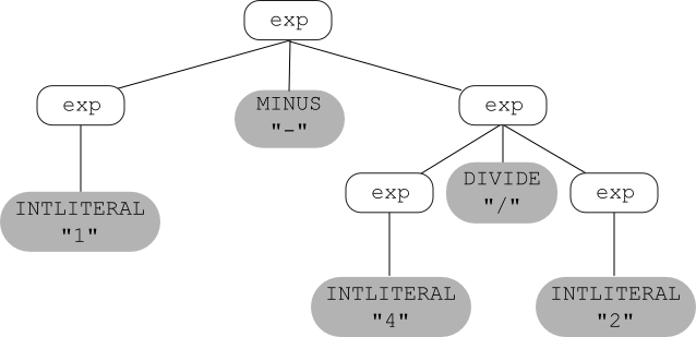
It should be readily apparent to you that the string is recognized by the the language, and can be produced via the (leftmost) derivation sequence:
Step #2. $\;\;\;\;\;\Longrightarrow$ intlit minus $Exp$ (via production P1)
Step #3. $\;\;\;\;\;\Longrightarrow$ intlit minus $Exp$ divide $Exp$ (via production P3)
Step #4. $\;\;\;\;\;\Longrightarrow$ intlit minus intlit divide $Exp$ (via production P1)
Step #5. $\;\;\;\;\;\Longrightarrow$ intlit minus intlit divide intlit (via production P1)
This derivation sequence corresponds to the parse tree:
However, inspection of the grammar also reveals that there is another leftmost derivation that can recognize the string by choosing to apply the rules differently:
Step #1. Exp $\Longrightarrow$ Exp divide Exp (via production P3)
Step #2. $\;\;\;\;\;\Longrightarrow$ Exp minus Exp divide Exp (via production P2)
Step #3. $\;\;\;\;\;\Longrightarrow$ intlit minus Exp divide Exp (via production P1)
Step #4. $\;\;\;\;\;\Longrightarrow$ intlit minus intlit divide Exp (via production P1)
Step #5. $\;\;\;\;\;\Longrightarrow$ intlit minus intlit divide intlit
(via production P1)
Which corresponds to the parse tree:
If for grammar $G$ and string $w$ there is:
then G is called an ambiguous grammar. (Note: the three conditions given above are equivalent; if one is true then all three are true.)
It is worth noting that ambiguity is not a problem for certain applications of Context-Free Grammars. As discussed in the intro, language recognition is satisfied by finding a one derivation for the string, and the string will certainly maintain membership in the language if there is more than one derivation possible. However, for the task of parsing, ambiguous grammars cause problems, both in the correctness of the parse tree and in the efficiency of building it. We will briefly explore both of these issues.
A problem of correctness: The major issue with ambiguous parse trees is that the underlying structure of the language is ill-defined. In the above example, subtraction and division can swap precedence; the first parse tree groups 4/2, while the second groups 1-4. These two groupings correspond to expressions with different values: the first tree corresponds to (1-(4/2)) and the second tree corresponds to ((1-4)/2).
A problem of efficiency: As we will see later, a parser can use significantly more efficient algorithms (in terms of Big-O complexity) by adding constraints to the language that it recognizes. One such assumption of some parsing algorithms is that the language recognized is unambiguous. To some extent, this issue can come up independently of correctness. For example, the following grammar has no issue of grouping (it only ever produces intlit), but production P1 can be applied any number of times before producing the integer literal token.
P2: Exp $\longrightarrow$ intlit
It's useful to know how to translate an ambiguous grammar into an equivalent unambiguous grammar Since every programming language includes expressions, we will discuss these operations in the context of an expression language. We are particularly interesting in forcing unambiguous precedence and associativies of the operators.
To write a grammar whose parse trees express precedence correctly, use a different nonterminal for each precedence level. Start by writing a rule for the operator(s) with the lowest precedence ("-" in our case), then write a rule for the operator(s) with the next lowest precedence, etc:
P2: Exp $\longrightarrow$ Term
P3: Term $\longrightarrow$ Term divide Term
P4: Term $\longrightarrow$ Factor
P5: Factor $\longrightarrow$ intlit
P6: Factor $\longrightarrow$ lparen Exp rparen
Now let's try using these new rules to build parse trees for
1 - 4 / 2.
First, a parse tree that correctly reflects that fact that division has higher precedence than subtraction:
Now we'll try to construct a parse tree that shows the wrong precedence:
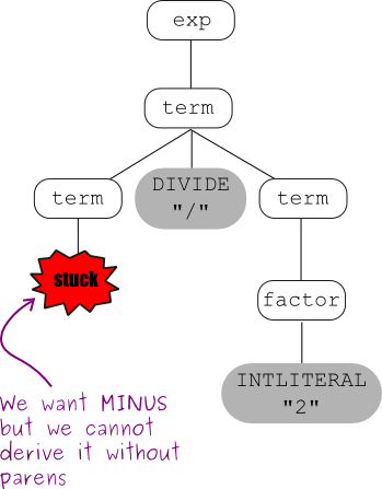
This grammar captures operator precedence, but it is still ambiguous! Parse trees using this grammar may not correctly express the fact that both subtraction and division are left associative; e.g., the expression: 5-3-2 is equivalent to: ((5-3)-2) and not to: (5-(3-2)).
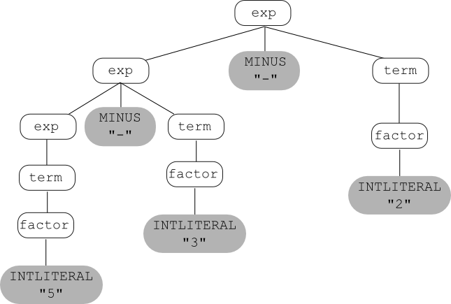
Draw two parse trees for the expression 5-3-2 using the current expression grammar:
-
exp → exp MINUS exp | term
term → term DIVIDE term | factor
factor → INTLITERAL | LPAREN exp RPAREN
To understand how to write expression grammars that correctly reflect the associativity of the operators, you need to understand about recursion in grammars.
The grammar given above for arithmetic expressions is both left and right recursive in nonterminals Exp and Term (try writing the derivation steps that show this).
To write a grammar that correctly expresses operator associativity:
Here's the correct grammar:
Term $\longrightarrow$ Term divide Factor | Factor
Factor $\longrightarrow$ intlit | lparen Exp rparen
And here's the (one and only) parse tree that can be built for 5 - 3 - 2 using this grammar:
Now let's consider a more complete expression grammar, for arithmetic expressions with addition, multiplication, and exponentiation, as well as subtraction and division. We'll use the token pow for the exponentiation operator, and we'll use "**" as the corresponding lexeme; e.g., "two to the third power" would be written: 2 ** 3, and the corresponding sequence of tokens would be: intlit pow intlit.
Here's an ambiguous context-free grammar for this language:
| Exp | $\longrightarrow$ | Exp plus Exp | Exp minus Exp | Exp times Exp | Exp divide Exp |
| | | Exp pow Exp | lparen Exp rparen | intlit |
First, we'll modify the grammar so that parse trees correctly reflect the fact that addition and subtraction have the same, lowest precedence; multiplication and division have the same, middle precedence; and exponentiation has the highest precedence:
| exp | → | exp PLUS exp | | exp MINUS exp | | term |
| term | → | term TIMES term | | term DIVIDE term | | factor |
| factor | → | factor POW factor | | exponent | |
| exponent | → | INTLITERAL | | LPAREN exp RPAREN |
This grammar is still ambiguous; it does not yet reflect the associativities of the operators. So next we'll modify the grammar so that parse trees correctly reflect the fact that all of the operators except exponentiation are left associative (and exponentiation is right associative; e.g., 2**3**4 is equivalent to: 2**(3**4)):
| exp | → exp PLUS term | | exp MINUS term | | term | ||
| term | → term TIMES factor | | term DIVIDE factor | | factor | ||
factor
| → exponent POW factor
| | exponent
| exponent
| → INTLITERAL
| | LPAREN exp RPAREN
| |
Finally, we'll modify the grammar by adding a unary operator, unary minus, which has the highest precedence of all (e.g., -3**4 is equivalent to: (-3)**4, not to -(3**4). Note that the notion of associativity does not apply to unary operators, since associativity only comes into play in an expression of the form: x op y op z.
| exp | → exp PLUS term | | exp MINUS term | | term | ||
| term | → term TIMES factor | | term DIVIDE factor | | factor | ||
| factor | → exponent POW factor | | exponent | |||
exponent
| → MINUS exponent
| | final
| final
| → INTLITERAL
| | LPAREN exp RPAREN
| |
Below is the grammar we used earlier for the language of boolean expressions, with two possible operands: true and false, and three possible operators: and, or, not:
BExp$\;\longrightarrow\;$false
BExp $\;\longrightarrow\;$ BExp or BExp
BExp $\;\longrightarrow\;$ BExp and BExp
BExp $\;\longrightarrow\;$ not BExp
BExp $\;\longrightarrow\;$ lparen BExp rparen
Question 1: Add nonterminals so that or has lowest precedence, then and, then not. Then change the grammar to reflect the fact that both and and or are left associative.
Question 2:
Draw a parse tree (using your final grammar for Question 1)
for the expression: true and not true.
Another kind of grammar that you will often need to write is a grammar that defines a list of something. There are several common forms. For each form given below, we provide three different grammars that define the specified list language.
A Grammar for a Programming Language
Using CFGs for programming language syntax has the notational advantage that the problem can be broken down into pieces. For example, let us begin sketching out a simple scripting language, that starts with productions for some top-level nonterminals:
| Program | $\longrightarrow$ | FunctionList |
| FunctionList | $\longrightarrow$ | Function | Function |